よく使われるデータ型
この章では、機械学習で最も一般的な4つのデータ型(数値型、テキスト型、画像型、カテゴリ型データ)を紹介します。
データ型は食材の種類のようなものです異なる食材には異なる処理方法が必要です。同様に、異なるタイプのデータにも異なる処理技術とアルゴリズムが必要です。
四大データ型の分類
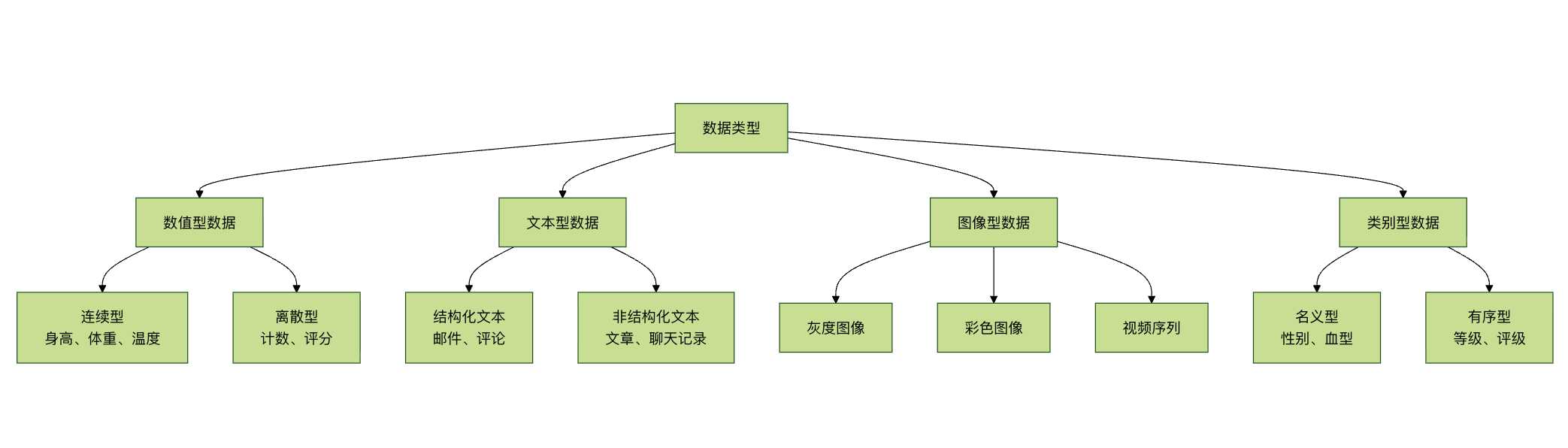
数値型データ
数値型データとは?
数値型データは、物差しで測定した結果のようなものです数学的な演算が可能で、機械学習で最も一般的なデータ型です。
数値型データの分類
1. 連続型数値データ
例
# 连续型数值数据示例
import numpy as np
import pandas as pd
import matplotlib.pyplot as plt
def continuous_data_example():
"""连续型数值数据示例"""
print("=== 连续型数值数据示例 ===")
# 生成连续型数据
np.random.seed(42)
n_samples = 1000
# 身高数据(连续型)
heights = np.random.normal(170, 10, n_samples) # 均值170,标准差10
weights = heights * 0.7 + np.random.normal(0, 5, n_samples) # 体重と身長の相関
temperatures = np.random.normal(36.5, 0.5, n_samples) # 体温
# 创建数据框
continuous_data = pd.DataFrame({
'身高(cm)': heights,
'体重(kg)': weights,
'体温(°C)': temperatures,
'年龄': np.random.randint(18, 65, n_samples)
})
print("连续型数据示例:")
print(continuous_data.head())
print(f"\n数据统计信息:")
print(continuous_data.describe())
# 可视化连续型数据分布
plt.figure(figsize=(12, 8))
plt.subplot(2, 2, 1)
plt.hist(continuous_data['身高(cm)'], bins=30, alpha=0.7, color='skyblue')
plt.title('身高分布')
plt.xlabel('身高 (cm)')
plt.ylabel('频数')
plt.subplot(2, 2, 2)
plt.hist(continuous_data['体重(kg)'], bins=30, alpha=0.7, color='lightgreen')
plt.title('体重分布')
plt.xlabel('体重 (kg)')
plt.ylabel('频数')
plt.subplot(2, 2, 3)
plt.hist(continuous_data['体温(°C)'], bins=30, alpha=0.7, color='salmon')
plt.title('体温分布')
plt.xlabel('体温 (°C)')
plt.ylabel('频数')
plt.subplot(2, 2, 4)
plt.scatter(continuous_data['身高(cm)'], continuous_data['体重(kg)'], alpha=0.6)
plt.title('身高 vs 体重')
plt.xlabel('身高 (cm)')
plt.ylabel('体重 (kg)')
plt.tight_layout()
plt.show()
return continuous_data
# 运行示例
continuous_df = continuous_data_example()
import numpy as np
import pandas as pd
import matplotlib.pyplot as plt
def continuous_data_example():
"""连续型数值数据示例"""
print("=== 连续型数值数据示例 ===")
# 生成连续型数据
np.random.seed(42)
n_samples = 1000
# 身高数据(连续型)
heights = np.random.normal(170, 10, n_samples) # 均值170,标准差10
weights = heights * 0.7 + np.random.normal(0, 5, n_samples) # 体重と身長の相関
temperatures = np.random.normal(36.5, 0.5, n_samples) # 体温
# 创建数据框
continuous_data = pd.DataFrame({
'身高(cm)': heights,
'体重(kg)': weights,
'体温(°C)': temperatures,
'年龄': np.random.randint(18, 65, n_samples)
})
print("连续型数据示例:")
print(continuous_data.head())
print(f"\n数据统计信息:")
print(continuous_data.describe())
# 可视化连续型数据分布
plt.figure(figsize=(12, 8))
plt.subplot(2, 2, 1)
plt.hist(continuous_data['身高(cm)'], bins=30, alpha=0.7, color='skyblue')
plt.title('身高分布')
plt.xlabel('身高 (cm)')
plt.ylabel('频数')
plt.subplot(2, 2, 2)
plt.hist(continuous_data['体重(kg)'], bins=30, alpha=0.7, color='lightgreen')
plt.title('体重分布')
plt.xlabel('体重 (kg)')
plt.ylabel('频数')
plt.subplot(2, 2, 3)
plt.hist(continuous_data['体温(°C)'], bins=30, alpha=0.7, color='salmon')
plt.title('体温分布')
plt.xlabel('体温 (°C)')
plt.ylabel('频数')
plt.subplot(2, 2, 4)
plt.scatter(continuous_data['身高(cm)'], continuous_data['体重(kg)'], alpha=0.6)
plt.title('身高 vs 体重')
plt.xlabel('身高 (cm)')
plt.ylabel('体重 (kg)')
plt.tight_layout()
plt.show()
return continuous_data
# 运行示例
continuous_df = continuous_data_example()
. 離散型数値データ
例
# 离散型数值数据示例
def discrete_data_example():
"""离散型数值数据示例"""
print("\n=== 离散型数值数据示例 ===")
# 生成离散型数据
np.random.seed(42)
n_samples = 500
# 离散型数据
customer_count = np.random.poisson(10, n_samples) # 泊松分布:顾客数量
product_rating = np.random.randint(1, 6, n_samples) # 1-5星评分
defect_count = np.random.binomial(20, 0.1, n_samples) # 二项分布:缺陷数量
call_duration = np.random.exponential(5, n_samples) * 60 # 指数分布:通话时长(秒)
# 创建数据框
discrete_data = pd.DataFrame({
'顾客数量': customer_count,
'产品评分': product_rating,
'缺陷数量': defect_count,
'通话时长(秒)': call_duration.astype(int)
})
print("离散型数据示例:")
print(discrete_data.head())
print(f"\n数据统计信息:")
print(discrete_data.describe())
# 可视化离散型数据
plt.figure(figsize=(12, 8))
plt.subplot(2, 2, 1)
plt.hist(discrete_data['顾客数量'], bins=range(0, max(discrete_data['顾客数量'])+2),
alpha=0.7, color='orange')
plt.title('顾客数量分布')
plt.xlabel('顾客数量')
plt.ylabel('频数')
plt.subplot(2, 2, 2)
value_counts = discrete_data['产品评分'].value_counts().sort_index()
plt.bar(value_counts.index, value_counts.values, color='purple', alpha=0.7)
plt.title('产品评分分布')
plt.xlabel('评分')
plt.ylabel('频数')
plt.subplot(2, 2, 3)
plt.hist(discrete_data['缺陷数量'], bins=range(0, max(discrete_data['缺陷数量'])+2),
alpha=0.7, color='red')
plt.title('缺陷数量分布')
plt.xlabel('缺陷数量')
plt.ylabel('频数')
plt.subplot(2, 2, 4)
plt.hist(discrete_data['通话时长(秒)'], bins=30, alpha=0.7, color='brown')
plt.title('通话时长分布')
plt.xlabel('通话时长 (秒)')
plt.ylabel('频数')
plt.tight_layout()
plt.show()
return discrete_data
# 运行示例
discrete_df = discrete_data_example()
def discrete_data_example():
"""离散型数值数据示例"""
print("\n=== 离散型数值数据示例 ===")
# 生成离散型数据
np.random.seed(42)
n_samples = 500
# 离散型数据
customer_count = np.random.poisson(10, n_samples) # 泊松分布:顾客数量
product_rating = np.random.randint(1, 6, n_samples) # 1-5星评分
defect_count = np.random.binomial(20, 0.1, n_samples) # 二项分布:缺陷数量
call_duration = np.random.exponential(5, n_samples) * 60 # 指数分布:通话时长(秒)
# 创建数据框
discrete_data = pd.DataFrame({
'顾客数量': customer_count,
'产品评分': product_rating,
'缺陷数量': defect_count,
'通话时长(秒)': call_duration.astype(int)
})
print("离散型数据示例:")
print(discrete_data.head())
print(f"\n数据统计信息:")
print(discrete_data.describe())
# 可视化离散型数据
plt.figure(figsize=(12, 8))
plt.subplot(2, 2, 1)
plt.hist(discrete_data['顾客数量'], bins=range(0, max(discrete_data['顾客数量'])+2),
alpha=0.7, color='orange')
plt.title('顾客数量分布')
plt.xlabel('顾客数量')
plt.ylabel('频数')
plt.subplot(2, 2, 2)
value_counts = discrete_data['产品评分'].value_counts().sort_index()
plt.bar(value_counts.index, value_counts.values, color='purple', alpha=0.7)
plt.title('产品评分分布')
plt.xlabel('评分')
plt.ylabel('频数')
plt.subplot(2, 2, 3)
plt.hist(discrete_data['缺陷数量'], bins=range(0, max(discrete_data['缺陷数量'])+2),
alpha=0.7, color='red')
plt.title('缺陷数量分布')
plt.xlabel('缺陷数量')
plt.ylabel('频数')
plt.subplot(2, 2, 4)
plt.hist(discrete_data['通话时长(秒)'], bins=30, alpha=0.7, color='brown')
plt.title('通话时长分布')
plt.xlabel('通话时长 (秒)')
plt.ylabel('频数')
plt.tight_layout()
plt.show()
return discrete_data
# 运行示例
discrete_df = discrete_data_example()
数値型データの処理方法
例
# 数值型数据处理方法
class NumericDataProcessor:
def __init__(self):
self.scalers = {}
self.transformers = {}
def detect_outliers(self, data, method='iqr'):
"""检测异常值"""
outliers_info = {}
for column in data.select_dtypes(include=[np.number]).columns:
if method == 'iqr':
Q1 = data[column].quantile(0.25)
Q3 = data[column].quantile(0.75)
IQR = Q3 - Q1
lower_bound = Q1 - 1.5 * IQR
upper_bound = Q3 + 1.5 * IQR
outliers = data[(data[column] < lower_bound) |
(data[column] > upper_bound)]
elif method == 'zscore':
z_scores = np.abs((data[column] - data[column].mean()) / data[column].std())
outliers = data[z_scores > 3]
outliers_info[column] = {
'count': len(outliers),
'indices': outliers.index.tolist(),
'percentage': (len(outliers) / len(data)) * 100
}
return outliers_info
def handle_missing_values(self, data, strategy='mean'):
"""处理缺失值"""
processed_data = data.copy()
for column in processed_data.select_dtypes(include=[np.number]).columns:
if processed_data[column].isnull().sum() > 0:
if strategy == 'mean':
processed_data[column].fillna(processed_data[column].mean(), inplace=True)
elif strategy == 'median':
processed_data[column].fillna(processed_data[column].median(), inplace=True)
elif strategy == 'mode':
processed_data[column].fillna(processed_data[column].mode()[0], inplace=True)
elif strategy == 'forward':
processed_data[column].fillna(method='ffill', inplace=True)
elif strategy == 'backward':
processed_data[column].fillna(method='bfill', inplace=True)
return processed_data
def normalize_data(self, data, method='minmax'):
"""数据标准化"""
from sklearn.preprocessing import MinMaxScaler, StandardScaler, RobustScaler
processed_data = data.copy()
numeric_columns = data.select_dtypes(include=[np.number]).columns
if method == 'minmax':
scaler = MinMaxScaler()
elif method == 'standard':
scaler = StandardScaler()
elif method == 'robust':
scaler = RobustScaler()
else:
raise ValueError("メソッドは 'minmax'、'standard'、または 'robust' でなければなりません。")
processed_data[numeric_columns] = scaler.fit_transform(processed_data[numeric_columns])
self.scalers[method] = scaler
return processed_data
def create_features(self, data):
"""特征工程"""
processed_data = data.copy()
numeric_columns = data.select_dtypes(include=[np.number]).columns
# 创建多项式特征
if len(numeric_columns) >= 2:
col1, col2 = numeric_columns[0], numeric_columns[1]
processed_data[f'{col1}_x_{col2}'] = data[col1] * data[col2]
processed_data[f'{col1}_div_{col2}'] = data[col1] / (data[col2] + 1e-8)
# 创建统计特征
for column in numeric_columns:
processed_data[f'{column}_log'] = np.log1p(data[column])
processed_data[f'{column}_sqrt'] = np.sqrt(np.abs(data[column]))
processed_data[f'{column}_square'] = data[column] ** 2
return processed_data
# 使用示例
processor = NumericDataProcessor()
# 检测异常值
outliers = processor.detect_outliers(continuous_df)
print("\n异常值检测结果:")
for column, info in outliers.items():
if info['count'] > 0:
print(f"{column}: {info['count']} 个异常值 ({info['percentage']:.2f}%)")
# 数据标准化
normalized_data = processor.normalize_data(continuous_df, method='standard')
print("\n標準化されたデータの例:)
print(normalized_data.head())
class NumericDataProcessor:
def __init__(self):
self.scalers = {}
self.transformers = {}
def detect_outliers(self, data, method='iqr'):
"""检测异常值"""
outliers_info = {}
for column in data.select_dtypes(include=[np.number]).columns:
if method == 'iqr':
Q1 = data[column].quantile(0.25)
Q3 = data[column].quantile(0.75)
IQR = Q3 - Q1
lower_bound = Q1 - 1.5 * IQR
upper_bound = Q3 + 1.5 * IQR
outliers = data[(data[column] < lower_bound) |
(data[column] > upper_bound)]
elif method == 'zscore':
z_scores = np.abs((data[column] - data[column].mean()) / data[column].std())
outliers = data[z_scores > 3]
outliers_info[column] = {
'count': len(outliers),
'indices': outliers.index.tolist(),
'percentage': (len(outliers) / len(data)) * 100
}
return outliers_info
def handle_missing_values(self, data, strategy='mean'):
"""处理缺失值"""
processed_data = data.copy()
for column in processed_data.select_dtypes(include=[np.number]).columns:
if processed_data[column].isnull().sum() > 0:
if strategy == 'mean':
processed_data[column].fillna(processed_data[column].mean(), inplace=True)
elif strategy == 'median':
processed_data[column].fillna(processed_data[column].median(), inplace=True)
elif strategy == 'mode':
processed_data[column].fillna(processed_data[column].mode()[0], inplace=True)
elif strategy == 'forward':
processed_data[column].fillna(method='ffill', inplace=True)
elif strategy == 'backward':
processed_data[column].fillna(method='bfill', inplace=True)
return processed_data
def normalize_data(self, data, method='minmax'):
"""数据标准化"""
from sklearn.preprocessing import MinMaxScaler, StandardScaler, RobustScaler
processed_data = data.copy()
numeric_columns = data.select_dtypes(include=[np.number]).columns
if method == 'minmax':
scaler = MinMaxScaler()
elif method == 'standard':
scaler = StandardScaler()
elif method == 'robust':
scaler = RobustScaler()
else:
raise ValueError("メソッドは 'minmax'、'standard'、または 'robust' でなければなりません。")
processed_data[numeric_columns] = scaler.fit_transform(processed_data[numeric_columns])
self.scalers[method] = scaler
return processed_data
def create_features(self, data):
"""特征工程"""
processed_data = data.copy()
numeric_columns = data.select_dtypes(include=[np.number]).columns
# 创建多项式特征
if len(numeric_columns) >= 2:
col1, col2 = numeric_columns[0], numeric_columns[1]
processed_data[f'{col1}_x_{col2}'] = data[col1] * data[col2]
processed_data[f'{col1}_div_{col2}'] = data[col1] / (data[col2] + 1e-8)
# 创建统计特征
for column in numeric_columns:
processed_data[f'{column}_log'] = np.log1p(data[column])
processed_data[f'{column}_sqrt'] = np.sqrt(np.abs(data[column]))
processed_data[f'{column}_square'] = data[column] ** 2
return processed_data
# 使用示例
processor = NumericDataProcessor()
# 检测异常值
outliers = processor.detect_outliers(continuous_df)
print("\n异常值检测结果:")
for column, info in outliers.items():
if info['count'] > 0:
print(f"{column}: {info['count']} 个异常值 ({info['percentage']:.2f}%)")
# 数据标准化
normalized_data = processor.normalize_data(continuous_df, method='standard')
print("\n標準化されたデータの例:)
print(normalized_data.head())
テキスト型データ
テキスト型データとは?
テキスト型データは、人間の言語による表現のようなものです豊かな意味情報を含んでいますが、機械学習モデルで使用するには特別な処理が必要です。
テキスト型データの分類
1. 構造化テキストデータ
例
# 结构化文本数据示例
import pandas as pd
import re
from collections import Counter
def structured_text_example():
"""结构化文本数据示例"""
print("\n=== 结构化文本数据示例 ===")
# 创建结构化文本数据
structured_data = pd.DataFrame({
'邮件ID': range(1, 11),
'发件人': [
'[email protected]', '[email protected]', '[email protected]',
'[email protected]', '[email protected]', '[email protected]',
'[email protected]', '[email protected]', '[email protected]',
'[email protected]'
],
'主题': [
'会议通知:明天下午3点开会',
'产品报价:最新价格表',
'客户反馈:服务满意度调查',
'项目进度:第一阶段完成',
'假期安排:国庆节放假通知',
'技术更新:系统升级公告',
'学术会议:论文征集通知',
'培训通知:新员工培训',
'政策文件:最新规定',
'健康提醒:体检通知'
],
'内容长度': [156, 234, 189, 145, 98, 267, 198, 134, 312, 87]
})
print("结构化文本数据示例:")
print(structured_data)
# 文本特征提取
print("\n=== 文本特征分析 ===")
# 邮箱域名分析
domains = [email.split('@')[1] for email in structured_data['发件人']]
domain_counts = Counter(domains)
print(f"邮箱域名分布:{dict(domain_counts)}")
# 主题关键词分析
all_words = []
for subject in structured_data['主题']:
words = re.findall(r'[\u4e00-\u9fff]+', subject) # 提取中文词汇
all_words.extend(words)
word_counts = Counter(all_words)
print(f"主题词频:{dict(word_counts)}")
# 内容长度统计
print(f"内容长度统计:")
print(structured_data['内容长度'].describe())
return structured_data
# 运行示例
structured_text_df = structured_text_example()
import pandas as pd
import re
from collections import Counter
def structured_text_example():
"""结构化文本数据示例"""
print("\n=== 结构化文本数据示例 ===")
# 创建结构化文本数据
structured_data = pd.DataFrame({
'邮件ID': range(1, 11),
'发件人': [
'[email protected]', '[email protected]', '[email protected]',
'[email protected]', '[email protected]', '[email protected]',
'[email protected]', '[email protected]', '[email protected]',
'[email protected]'
],
'主题': [
'会议通知:明天下午3点开会',
'产品报价:最新价格表',
'客户反馈:服务满意度调查',
'项目进度:第一阶段完成',
'假期安排:国庆节放假通知',
'技术更新:系统升级公告',
'学术会议:论文征集通知',
'培训通知:新员工培训',
'政策文件:最新规定',
'健康提醒:体检通知'
],
'内容长度': [156, 234, 189, 145, 98, 267, 198, 134, 312, 87]
})
print("结构化文本数据示例:")
print(structured_data)
# 文本特征提取
print("\n=== 文本特征分析 ===")
# 邮箱域名分析
domains = [email.split('@')[1] for email in structured_data['发件人']]
domain_counts = Counter(domains)
print(f"邮箱域名分布:{dict(domain_counts)}")
# 主题关键词分析
all_words = []
for subject in structured_data['主题']:
words = re.findall(r'[\u4e00-\u9fff]+', subject) # 提取中文词汇
all_words.extend(words)
word_counts = Counter(all_words)
print(f"主题词频:{dict(word_counts)}")
# 内容长度统计
print(f"内容长度统计:")
print(structured_data['内容长度'].describe())
return structured_data
# 运行示例
structured_text_df = structured_text_example()
2. 非構造化テキストデータ
例
# 非结构化文本数据示例
def unstructured_text_example():
"""非结构化文本数据示例"""
print("\n=== 非结构化文本数据示例 ===")
# 创建非结构化文本数据
unstructured_texts = [
"""
人工知能技術は急速に発展しており、深層学習、機械学習、自然言語処理などの分野で大きな進歩が遂げられています。
これらの技術は、医療、金融、教育、交通などの多くの業界で広く応用されており、社会の発展に新たな機会をもたらしています。
将来、計算能力の向上とアルゴリズムの改善に伴い、人工知能はより多くの分野で重要な役割を果たすでしょう。
""",
"""
今日は天気がとても良く、日差しが明るく、そよ風が吹いています。私は公園を散歩して、この素晴らしい時間を楽しむことにしました。
公園にはたくさんの花があります。赤い花、黄色い花、紫の花など、色とりどりでとても美しいです。小鳥が木の上で歌っています。
蝶が花々の間を舞い、すべてがとても調和ので自然に見える。
""",
"""
株式市場は今日は力強い動きを見せ、上海総合指数は2.3%上昇、深セン成分指数は1.8%上昇した。
ハイテク株が上昇をけん引し、多くの銘柄がストップ高となった。アナリストは、これは主に最近発表された好材料の政策によるものとみている。
投資家の信頼感が高まり、市場の売買は活発化し、出来高は明らかに膨らんだ。
""",
"""
健康的な生活様式には、バランスの取れた食事、適度な運動、十分な睡眠、良好な心構えが含まれる。
毎日野菜や果物を摂取し、油っこい食べ物を減らすことを勧める。毎週少なくとも3回、毎回30分以上運動する。
7〜8時間の睡眠を確保する。感情をコントロールすることを学び、前向きで楽観的な心構えを保つ。
"""
]
text_categories = ['テクノロジー', '生活', '経済', '健康']
# データフレームを作成
unstructured_df = pd.DataFrame({
'テキスト': unstructured_texts,
'カテゴリ': text_categories
})
print("非構造化テキストデータの例:")
for i, row in unstructured_df.iterrows():
print(f"\nカテゴリ:{row['类别']}")
print(f"テキスト:{row['文本'][:100]}...")
return unstructured_df
# サンプルを実行
unstructured_text_df = unstructured_text_example()
def unstructured_text_example():
"""非结构化文本数据示例"""
print("\n=== 非结构化文本数据示例 ===")
# 创建非结构化文本数据
unstructured_texts = [
"""
人工知能技術は急速に発展しており、深層学習、機械学習、自然言語処理などの分野で大きな進歩が遂げられています。
これらの技術は、医療、金融、教育、交通などの多くの業界で広く応用されており、社会の発展に新たな機会をもたらしています。
将来、計算能力の向上とアルゴリズムの改善に伴い、人工知能はより多くの分野で重要な役割を果たすでしょう。
""",
"""
今日は天気がとても良く、日差しが明るく、そよ風が吹いています。私は公園を散歩して、この素晴らしい時間を楽しむことにしました。
公園にはたくさんの花があります。赤い花、黄色い花、紫の花など、色とりどりでとても美しいです。小鳥が木の上で歌っています。
蝶が花々の間を舞い、すべてがとても調和ので自然に見える。
""",
"""
株式市場は今日は力強い動きを見せ、上海総合指数は2.3%上昇、深セン成分指数は1.8%上昇した。
ハイテク株が上昇をけん引し、多くの銘柄がストップ高となった。アナリストは、これは主に最近発表された好材料の政策によるものとみている。
投資家の信頼感が高まり、市場の売買は活発化し、出来高は明らかに膨らんだ。
""",
"""
健康的な生活様式には、バランスの取れた食事、適度な運動、十分な睡眠、良好な心構えが含まれる。
毎日野菜や果物を摂取し、油っこい食べ物を減らすことを勧める。毎週少なくとも3回、毎回30分以上運動する。
7〜8時間の睡眠を確保する。感情をコントロールすることを学び、前向きで楽観的な心構えを保つ。
"""
]
text_categories = ['テクノロジー', '生活', '経済', '健康']
# データフレームを作成
unstructured_df = pd.DataFrame({
'テキスト': unstructured_texts,
'カテゴリ': text_categories
})
print("非構造化テキストデータの例:")
for i, row in unstructured_df.iterrows():
print(f"\nカテゴリ:{row['类别']}")
print(f"テキスト:{row['文本'][:100]}...")
return unstructured_df
# サンプルを実行
unstructured_text_df = unstructured_text_example()
テキストデータの処理方法
例
# テキストデータ処理方法
import jieba
from sklearn.feature_extraction.text import TfidfVectorizer, CountVectorizer
from sklearn.preprocessing import LabelEncoder
class TextDataProcessor:
def __init__(self):
self.vectorizers = {}
self.label_encoders = {}
def clean_text(self, text):
"""テキストクリーニング"""
# 特殊文字と数字を削除する
text = re.sub(r'[^\u4e00-\u9fff\s]', '', text)
# 余分な空白を削除する
text = re.sub(r'\s+', ' ', text).strip()
return text
def tokenize_chinese(self, text):
"""中国語の分かち書き"""
words = jieba.lcut(text)
# ストップワードを削除(簡易版)
stop_words = {'の', 'た', 'に', 'だ', '我', '有', 'と', '就', '不', '人', '都', '一', '一个', '上', '也', '很', '到', '说', '要', '去', '你', '会', 'ている', '没有', '看', '好', '自己', 'これ'}
words = [word for word in words if word not in stop_words and len(word) > 1]
return words
def extract_features(self, texts, method='tfidf'):
"""特徴抽出"""
# テキストの前処理
cleaned_texts = [self.clean_text(text) for text in texts]
if method == 'tfidf':
vectorizer = TfidfVectorizer(max_features=1000, token_pattern=r'(?u)\b\w+\b')
elif method == 'count':
vectorizer = CountVectorizer(max_features=1000, token_pattern=r'(?u)\b\w+\b')
else:
raise ValueError("メソッドは 'tfidf' または 'count' でなければなりません")
features = vectorizer.fit_transform(cleaned_texts)
self.vectorizers[method] = vectorizer
return features.toarray(), vectorizer.get_feature_names_out()
def analyze_text_statistics(self, texts):
"""テキスト統計分析"""
stats = []
for text in texts:
cleaned_text = self.clean_text(text)
words = self.tokenize_chinese(cleaned_text)
stats.append({
'文字数': len(text),
'クリーニング後の文字数': len(cleaned_text),
'単語数': len(words),
'平均単語長': np.mean([len(word) for word in words]) if words else 0,
'異なり単語数': len(set(words))
})
return pd.DataFrame(stats)
def encode_labels(self, labels):
"""ラベルエンコーディング"""
encoder = LabelEncoder()
encoded_labels = encoder.fit_transform(labels)
self.label_encoders['default'] = encoder
return encoded_labels, encoder.classes_
# 使用例
text_processor = TextDataProcessor()
# テキスト統計分析
text_stats = text_processor.analyze_text_statistics(unstructured_text_df['テキスト'])
print("\nテキスト統計分析:")
print(text_stats)
# 特徴抽出
features, feature_names = text_processor.extract_features(
unstructured_text_df['テキスト'], method='tfidf'
)
print(f"\n特徴行列の形状:{features.shape}")
print(f"最初の10個の特徴:{feature_names[:10]}")
# ラベルエンコーディング
encoded_labels, label_classes = text_processor.encode_labels(
unstructured_text_df['カテゴリ']
)
print(f"\nエンコード後のラベル:{encoded_labels}")
print(f"ラベルのカテゴリ:{label_classes}")
画像型データ
画像型データとは?
画像型データは、視覚世界のデジタル化された表現のようなものです、ピクセル点で構成され、豊富な空間情報と色情報を含みます。
画像型データの分類
1. グレースケール画像
例
# グレースケール画像の例
import numpy as np
import matplotlib.pyplot as plt
from PIL import Image
def grayscale_image_example():
"""グレースケール画像の例"""
print("\n=== グレースケール画像の例 ===)
# シンプルなグレースケール画像を作成
# 100x100 のグレースケール画像を作成
height, width = 100, 100
# グラデーション画像を作成
gradient = np.zeros((height, width))
for i in range(height):
gradient[i, :] = i # 垂直グラデーション
# チェッカーボードパターンを作成
checkerboard = np.zeros((height, width))
for i in range(0, height, 10):
for j in range(0, width, 10):
if (i // 10 + j // 10) % 2 == 0:
checkerboard[i:i+10, j:j+10] = 255
# 円形パターンを作成
circle = np.zeros((height, width))
center_x, center_y = width // 2, height // 2
radius = 30
for i in range(height):
for j in range(width):
if (i - center_y) ** 2 + (j - center_x) ** 2 <= radius ** 2:
circle[i, j] = 255
# 画像を表示
plt.figure(figsize=(12, 4))
plt.subplot(1, 3, 1)
plt.imshow(gradient, cmap='gray')
plt.title('グラデーション画像')
plt.axis('off')
plt.subplot(1, 3, 2)
plt.imshow(checkerboard, cmap='gray')
plt.title('チェッカーボードパターン')
plt.axis('off')
plt.subplot(1, 3, 3)
plt.imshow(circle, cmap='gray')
plt.title('円形パターン')
plt.axis('off')
plt.tight_layout()
plt.show()
# 画像データ情報
print(f"グラデーション画像の形状:{gradient.shape}")
print(f"データ型:{gradient.dtype}")
print(f"ピクセル値の範囲:{gradient.min()} - {gradient.max()}")
return gradient, checkerboard, circle
# サンプルを実行
gradient_img, checkerboard_img, circle_img = grayscale_image_example()
import numpy as np
import matplotlib.pyplot as plt
from PIL import Image
def grayscale_image_example():
"""グレースケール画像の例"""
print("\n=== グレースケール画像の例 ===)
# シンプルなグレースケール画像を作成
# 100x100 のグレースケール画像を作成
height, width = 100, 100
# グラデーション画像を作成
gradient = np.zeros((height, width))
for i in range(height):
gradient[i, :] = i # 垂直グラデーション
# チェッカーボードパターンを作成
checkerboard = np.zeros((height, width))
for i in range(0, height, 10):
for j in range(0, width, 10):
if (i // 10 + j // 10) % 2 == 0:
checkerboard[i:i+10, j:j+10] = 255
# 円形パターンを作成
circle = np.zeros((height, width))
center_x, center_y = width // 2, height // 2
radius = 30
for i in range(height):
for j in range(width):
if (i - center_y) ** 2 + (j - center_x) ** 2 <= radius ** 2:
circle[i, j] = 255
# 画像を表示
plt.figure(figsize=(12, 4))
plt.subplot(1, 3, 1)
plt.imshow(gradient, cmap='gray')
plt.title('グラデーション画像')
plt.axis('off')
plt.subplot(1, 3, 2)
plt.imshow(checkerboard, cmap='gray')
plt.title('チェッカーボードパターン')
plt.axis('off')
plt.subplot(1, 3, 3)
plt.imshow(circle, cmap='gray')
plt.title('円形パターン')
plt.axis('off')
plt.tight_layout()
plt.show()
# 画像データ情報
print(f"グラデーション画像の形状:{gradient.shape}")
print(f"データ型:{gradient.dtype}")
print(f"ピクセル値の範囲:{gradient.min()} - {gradient.max()}")
return gradient, checkerboard, circle
# サンプルを実行
gradient_img, checkerboard_img, circle_img = grayscale_image_example()
2. カラー画像
例
# カラー画像の例
def color_image_example():
"""カラー画像の例"""
print("\n=== カラー画像の例 ===)
height, width = 100, 100
# RGB カラー画像を作成
# 赤のグラデーション
red_gradient = np.zeros((height, width, 3), dtype=np.uint8)
red_gradient[:, :, 0] = np.linspace(0, 255, width) # 赤チャンネルのグラデーション
# 緑のグラデーション
green_gradient = np.zeros((height, width, 3), dtype=np.uint8)
green_gradient[:, :, 1] = np.linspace(0, 255, width) # 緑チャンネルのグラデーション
# 青のグラデーション
blue_gradient = np.zeros((height, width, 3), dtype=np.uint8)
blue_gradient[:, :, 2] = np.linspace(0, 255, width) # 青チャンネルのグラデーション
# 虹色パターン
rainbow = np.zeros((height, width, 3), dtype=np.uint8)
for i in range(width):
hue = i / width
# 簡易版の HSV から RGB への変換
if hue < 1/3:
rainbow[:, i] = [255 * (1 - 3*hue), 255 * 3*hue, 0]
elif hue < 2/3:
rainbow[:, i] = [0, 255 * (2 - 3*hue), 255 * (3*hue - 1)]
else:
rainbow[:, i] = [255 * (3*hue - 2), 0, 255 * (3 - 3*hue)]
# 画像を表示
plt.figure(figsize=(12, 8))
plt.subplot(2, 2, 1)
plt.imshow(red_gradient)
plt.title('赤のグラデーション')
plt.axis('off')
plt.subplot(2, 2, 2)
plt.imshow(green_gradient)
plt.title('緑のグラデーション')
plt.axis('off')
plt.subplot(2, 2, 3)
plt.imshow(blue_gradient)
plt.title('青のグラデーション')
plt.axis('off')
plt.subplot(2, 2, 4)
plt.imshow(rainbow)
plt.title('虹色パターン')
plt.axis('off')
plt.tight_layout()
plt.show()
# 画像チャンネル情報
print(f"カラー画像の形状:{rainbow.shape}")
print(f"データ型:{rainbow.dtype}")
print(f"ピクセル値の範囲:{rainbow.min()} - {rainbow.max()}")
return red_gradient, green_gradient, blue_gradient, rainbow
# サンプルを実行
red_img, green_img, blue_img, rainbow_img = color_image_example()
def color_image_example():
"""カラー画像の例"""
print("\n=== カラー画像の例 ===)
height, width = 100, 100
# RGB カラー画像を作成
# 赤のグラデーション
red_gradient = np.zeros((height, width, 3), dtype=np.uint8)
red_gradient[:, :, 0] = np.linspace(0, 255, width) # 赤チャンネルのグラデーション
# 緑のグラデーション
green_gradient = np.zeros((height, width, 3), dtype=np.uint8)
green_gradient[:, :, 1] = np.linspace(0, 255, width) # 緑チャンネルのグラデーション
# 青のグラデーション
blue_gradient = np.zeros((height, width, 3), dtype=np.uint8)
blue_gradient[:, :, 2] = np.linspace(0, 255, width) # 青チャンネルのグラデーション
# 虹色パターン
rainbow = np.zeros((height, width, 3), dtype=np.uint8)
for i in range(width):
hue = i / width
# 簡易版の HSV から RGB への変換
if hue < 1/3:
rainbow[:, i] = [255 * (1 - 3*hue), 255 * 3*hue, 0]
elif hue < 2/3:
rainbow[:, i] = [0, 255 * (2 - 3*hue), 255 * (3*hue - 1)]
else:
rainbow[:, i] = [255 * (3*hue - 2), 0, 255 * (3 - 3*hue)]
# 画像を表示
plt.figure(figsize=(12, 8))
plt.subplot(2, 2, 1)
plt.imshow(red_gradient)
plt.title('赤のグラデーション')
plt.axis('off')
plt.subplot(2, 2, 2)
plt.imshow(green_gradient)
plt.title('緑のグラデーション')
plt.axis('off')
plt.subplot(2, 2, 3)
plt.imshow(blue_gradient)
plt.title('青のグラデーション')
plt.axis('off')
plt.subplot(2, 2, 4)
plt.imshow(rainbow)
plt.title('虹色パターン')
plt.axis('off')
plt.tight_layout()
plt.show()
# 画像チャンネル情報
print(f"カラー画像の形状:{rainbow.shape}")
print(f"データ型:{rainbow.dtype}")
print(f"ピクセル値の範囲:{rainbow.min()} - {rainbow.max()}")
return red_gradient, green_gradient, blue_gradient, rainbow
# サンプルを実行
red_img, green_img, blue_img, rainbow_img = color_image_example()
画像データの処理方法
例
# 画像データ処理方法
from skimage import filters, feature, measure, transform
from skimage.color import rgb2gray, rgb2hsv
class ImageDataProcessor:
def __init__(self):
pass
def resize_image(self, image, target_size):
"""画像サイズの調整"""
from skimage.transform import resize
return resize(image, target_size, anti_aliasing=True)
def normalize_image(self, image):
"""画像の正規化"""
return (image - image.min()) / (image.max() - image.min())
def extract_color_features(self, image):
"""色特徴の抽出"""
if len(image.shape) == 3: # カラー画像
# 各チャンネルの統計的特徴を計算する
features = {}
for i, channel in enumerate(['R', 'G', 'B']):
channel_data = image[:, :, i]
features[f'{channel}_mean'] = np.mean(channel_data)
features[f'{channel}_std'] = np.std(channel_data)
features[f'{channel}_min'] = np.min(channel_data)
features[f'{channel}_max'] = np.max(channel_data)
# 色ヒストグラムの特徴を計算する
hist_r, _ = np.histogram(image[:, :, 0], bins=256, range=(0, 256))
hist_g, _ = np.histogram(image[:, :, 1], bins=256, range=(0, 256))
hist_b, _ = np.histogram(image[:, :, 2], bins=256, range=(0, 256))
features.update({
'hist_r_peak': np.argmax(hist_r),
'hist_g_peak': np.argmax(hist_g),
'hist_b_peak': np.argmax(hist_b)
})
return features
else: # グレースケール画像
return {
'mean': np.mean(image),
'std': np.std(image),
'min': np.min(image),
'max': np.max(image)
}
def extract_texture_features(self, image):
"""テクスチャ特徴の抽出"""
if len(image.shape) == 3:
image = rgb2gray(image)
# エッジ特徴を計算する
edges = filters.sobel(image)
edge_density = np.sum(edges > 0) / edges.size
# 局所二値パターンを計算(簡易版)
lbp = feature.local_binary_pattern(image, P=8, R=1, method='uniform')
lbp_hist, _ = np.histogram(lbp.ravel(), bins=10)
return {
'edge_density': edge_density,
'lbp_hist': lbp_hist.tolist()
}
def augment_image(self, image):
"""画像拡張"""
augmented = []
# 元画像
augmented.append(image)
# 水平に反転
augmented.append(np.fliplr(image))
# 垂直に反転
augmented.append(np.flipud(image))
# 90度回転
augmented.append(np.rot90(image))
# 明るさを調整
if len(image.shape) == 3:
brightened = np.clip(image * 1.2, 0, 255).astype(np.uint8)
else:
brightened = np.clip(image * 1.2, 0, 1)
augmented.append(brightened)
return augmented
def visualize_image_channels(self, image):
"""画像チャンネルの可視化"""
if len(image.shape) == 3:
plt.figure(figsize=(12, 3))
plt.subplot(1, 4, 1)
plt.imshow(image)
plt.title('元画像')
plt.axis('off')
plt.subplot(1, 4, 2)
plt.imshow(image[:, :, 0], cmap='Reds')
plt.title('赤チャンネル')
plt.axis('off')
plt.subplot(1, 4, 3)
plt.imshow(image[:, :, 1], cmap='Greens')
plt.title('緑チャンネル')
plt.axis('off')
plt.subplot(1, 4, 4)
plt.imshow(image[:, :, 2], cmap='Blues')
plt.title('青チャンネル')
plt.axis('off')
plt.tight_layout()
plt.show()
# 使用例
image_processor = ImageDataProcessor()
# 色特徴を抽出
color_features = image_processor.extract_color_features(rainbow_img)
print("\n色特徴:")
for key, value in color_features.items():
if not key.startswith('hist'):
print(f"{key}: {value:.2f}")
# テクスチャ特徴を抽出
texture_features = image_processor.extract_texture_features(checkerboard_img)
print("\nテクスチャ特徴:")
for key, value in texture_features.items():
if key != 'lbp_hist':
print(f"{key}: {value:.4f}")
# 画像拡張
augmented_images = image_processor.augment_image(circle_img)
print(f"\n画像拡張:{len(augmented_images)} 個のバリアントを生成しました")
# 画像チャンネルを可視化
image_processor.visualize_image_channels(rainbow_img)
カテゴリ型データ
カテゴリ型データとは?
カテゴリ型データは分類ラベルのようなものです、異なるカテゴリやグループを表し、数学的演算はできません。
カテゴリ型データの分類
1. 名義型データ
例
# 名義型データの例
def nominal_data_example():
"""名義型データの例"""
print("\n=== 名義型データの例 ===)
# 名義型データを作成
nominal_data = pd.DataFrame({
'学生ID': range(1, 11),
'氏名': ['张三', '李四', '王五', '赵六', '钱七', '孙八', '周九', '吴十', '郑十一', '陈十二'],
'性別': ['男', '女', '男', '男', '女', '女', '男', '女', '男', '女'],
'血液型': ['A', 'B', 'O', 'AB', 'A', 'B', 'O', 'AB', 'A', 'O'],
'都市': ['北京', '上海', '広州', '深セン', '北京', '上海', '広州', '深セン', '北京', '上海'],
'専攻': ['コンピュータ', '数学', '物理', '化学', 'コンピュータ', '数学', '物理', '化学', 'コンピュータ', '数学']
})
print("名義型データの例:")
print(nominal_data)
# カテゴリ統計分析
print("\n=== カテゴリ統計分析 ===)
for column in nominal_data.select_dtypes(include=['object']).columns:
if column != '氏名': # 氏名列をスキップ
value_counts = nominal_data[column].value_counts()
print(f"\n{column} 分布:")
print(value_counts)
print(f"一意の値の数:{len(value_counts)}")
return nominal_data
# 実行例
nominal_df = nominal_data_example()
def nominal_data_example():
"""名義型データの例"""
print("\n=== 名義型データの例 ===)
# 名義型データを作成
nominal_data = pd.DataFrame({
'学生ID': range(1, 11),
'氏名': ['张三', '李四', '王五', '赵六', '钱七', '孙八', '周九', '吴十', '郑十一', '陈十二'],
'性別': ['男', '女', '男', '男', '女', '女', '男', '女', '男', '女'],
'血液型': ['A', 'B', 'O', 'AB', 'A', 'B', 'O', 'AB', 'A', 'O'],
'都市': ['北京', '上海', '広州', '深セン', '北京', '上海', '広州', '深セン', '北京', '上海'],
'専攻': ['コンピュータ', '数学', '物理', '化学', 'コンピュータ', '数学', '物理', '化学', 'コンピュータ', '数学']
})
print("名義型データの例:")
print(nominal_data)
# カテゴリ統計分析
print("\n=== カテゴリ統計分析 ===)
for column in nominal_data.select_dtypes(include=['object']).columns:
if column != '氏名': # 氏名列をスキップ
value_counts = nominal_data[column].value_counts()
print(f"\n{column} 分布:")
print(value_counts)
print(f"一意の値の数:{len(value_counts)}")
return nominal_data
# 実行例
nominal_df = nominal_data_example()
2. 順序型データ
例
# 順序型データの例
def ordinal_data_example():
"""順序型データの例"""
print("\n=== 順序型データの例 ===)
# 順序型データを作成
ordinal_data = pd.DataFrame({
'製品ID': range(1, 11),
'製品名': [f'製品{i}' for i in range(1, 11)],
'品質等級': ['優秀', '良好', '普通', '優秀', '良好', '普通', '不良', '優秀', '良好', '普通'],
'顧客満足度': ['非常に満足', '満足', '普通', '非常に満足', '満足', '普通', '不満', '非常に満足', '満足', '普通'],
'価格帯': ['高', '中', '低', '高', '中', '低', '低', '高', '中', '中'],
'売上ランキング': [1, 3, 5, 2, 4, 7, 9, 6, 8, 10]
})
print("順序型データの例:")
print(ordinal_data)
# 順序データの統計分析
print("\n=== 順序データの統計分析 ===)
# 順序を定義
quality_order = ['不良', '普通', '良好', '優秀']
satisfaction_order = ['不満', '普通', '満足', '非常に満足']
price_order = ['低', '中', '高']
# 順序カテゴリに変換
ordinal_data['品質等級_順序'] = pd.Categorical(
ordinal_data['品質等級'], categories=quality_order, ordered=True
)
ordinal_data['顧客満足度_順序'] = pd.Categorical(
ordinal_data['顧客満足度'], categories=satisfaction_order, ordered=True
)
ordinal_data['価格帯_順序'] = pd.Categorical(
ordinal_data['価格帯'], categories=price_order, ordered=True
)
# 統計分析
for column in ['品質等級_順序', '顧客満足度_順序', '価格帯_順序']:
print(f"\n{column} 分布:")
value_counts = ordinal_data[column].value_counts().sort_index()
print(value_counts)
# 中央値を計算
median_value = ordinal_data[column].median()
print(f"中央値:{median_value}")
return ordinal_data
# 実行例
ordinal_df = ordinal_data_example()
def ordinal_data_example():
"""順序型データの例"""
print("\n=== 順序型データの例 ===)
# 順序型データを作成
ordinal_data = pd.DataFrame({
'製品ID': range(1, 11),
'製品名': [f'製品{i}' for i in range(1, 11)],
'品質等級': ['優秀', '良好', '普通', '優秀', '良好', '普通', '不良', '優秀', '良好', '普通'],
'顧客満足度': ['非常に満足', '満足', '普通', '非常に満足', '満足', '普通', '不満', '非常に満足', '満足', '普通'],
'価格帯': ['高', '中', '低', '高', '中', '低', '低', '高', '中', '中'],
'売上ランキング': [1, 3, 5, 2, 4, 7, 9, 6, 8, 10]
})
print("順序型データの例:")
print(ordinal_data)
# 順序データの統計分析
print("\n=== 順序データの統計分析 ===)
# 順序を定義
quality_order = ['不良', '普通', '良好', '優秀']
satisfaction_order = ['不満', '普通', '満足', '非常に満足']
price_order = ['低', '中', '高']
# 順序カテゴリに変換
ordinal_data['品質等級_順序'] = pd.Categorical(
ordinal_data['品質等級'], categories=quality_order, ordered=True
)
ordinal_data['顧客満足度_順序'] = pd.Categorical(
ordinal_data['顧客満足度'], categories=satisfaction_order, ordered=True
)
ordinal_data['価格帯_順序'] = pd.Categorical(
ordinal_data['価格帯'], categories=price_order, ordered=True
)
# 統計分析
for column in ['品質等級_順序', '顧客満足度_順序', '価格帯_順序']:
print(f"\n{column} 分布:")
value_counts = ordinal_data[column].value_counts().sort_index()
print(value_counts)
# 中央値を計算
median_value = ordinal_data[column].median()
print(f"中央値:{median_value}")
return ordinal_data
# 実行例
ordinal_df = ordinal_data_example()
カテゴリ型データの処理方法
例
# カテゴリ型データの処理方法
from sklearn.preprocessing import LabelEncoder, OneHotEncoder, OrdinalEncoder
class CategoricalDataProcessor:
def __init__(self):
self.encoders = {}
self.feature_names = {}
def label_encoding(self, data, columns):
"""ラベルエンコーディング"""
encoded_data = data.copy()
for column in columns:
encoder = LabelEncoder()
encoded_data[f'{column}_encoded'] = encoder.fit_transform(data[column])
self.encoders[f'{column}_label'] = encoder
print(f"{column} ラベルエンコーディング:")
for i, category in enumerate(encoder.classes_):
print(f" {category} -> {i}")
return encoded_data
def one_hot_encoding(self, data, columns):
"""ワンホットエンコーディング"""
encoded_data = data.copy()
for column in columns:
encoder = OneHotEncoder(sparse=False, drop='first') # 多重共線性を回避
encoded_features = encoder.fit_transform(data[[column]])
# 新しい列名を作成
feature_names = [f'{column}_{category}' for category in encoder.categories_[0][1:]]
# データフレームに追加
for i, feature_name in enumerate(feature_names):
encoded_data[feature_name] = encoded_features[:, i]
self.encoders[f'{column}_onehot'] = encoder
self.feature_names[f'{column}_onehot'] = feature_names
print(f"{column} ワンホットエンコーディング:{len(feature_names)} 個の特徴を作成しました")
return encoded_data
def ordinal_encoding(self, data, columns, categories_list):
"""順序エンコーディング"""
encoded_data = data.copy()
for column, categories in zip(columns, categories_list):
encoder = OrdinalEncoder(categories=[categories])
encoded_data[f'{column}_ordinal'] = encoder.fit_transform(data[[column]])
self.encoders[f'{column}_ordinal'] = encoder
print(f"{column} 順序エンコーディング:")
for i, category in enumerate(categories):
print(f" {category} -> {i}")
return encoded_data
def target_encoding(self, data, categorical_column, target_column):
"""ターゲットエンコーディング"""
encoded_data = data.copy()
# 各カテゴリのターゲット平均を計算
target_means = data.groupby(categorical_column)[target_column].mean()
# エンコーディングを適用
encoded_data[f'{categorical_column}_target'] = data[categorical_column].map(target_means)
print(f"{categorical_column} ターゲットエンコーディング:")
for category, mean_value in target_means.items():
print(f" {category} -> {mean_value:.4f}")
return encoded_data
def frequency_encoding(self, data, columns):
"""頻度エンコーディング"""
encoded_data = data.copy()
for column in columns:
# 各カテゴリの頻度を計算
frequency = data[column].value_counts(normalize=True)
# エンコーディングを適用
encoded_data[f'{column}_frequency'] = data[column].map(frequency)
print(f"{column} 頻度エンコーディング:")
for category, freq in frequency.head().items():
print(f" {category} -> {freq:.4f}")
return encoded_data
def analyze_categorical_importance(self, data, categorical_columns, target_column):
"""カテゴリ特徴量の重要度を分析"""
importance_scores = {}
for column in categorical_columns:
# 各カテゴリのターゲット平均差を計算
category_means = data.groupby(column)[target_column].mean()
mean_difference = category_means.max() - category_means.min()
# カテゴリ数を計算
unique_count = data[column].nunique()
# 簡易な重要度スコア
importance = mean_difference * np.log(unique_count + 1)
importance_scores[column] = importance
# 並べ替え
sorted_importance = sorted(importance_scores.items(), key=lambda x: x[1], reverse=True)
print("\nカテゴリ特徴量の重要度:")
for column, importance in sorted_importance:
print(f"{column}: {importance:.4f}")
return importance_scores
# 使用例
cat_processor = CategoricalDataProcessor()
# 名義型データに数値ターゲットを追加
nominal_df_with_target = nominal_df.copy()
nominal_df_with_target['成績'] = np.random.randint(60, 100, len(nominal_df))
# ラベルエンコーディング
label_encoded = cat_processor.label_encoding(
nominal_df_with_target, ['性別', '血液型', '都市']
)
# ワンホットエンコーディング
onehot_encoded = cat_processor.one_hot_encoding(
nominal_df_with_target, ['専攻']
)
# ターゲットエンコーディング
target_encoded = cat_processor.target_encoding(
nominal_df_with_target, '都市', '成績'
)
# 頻度エンコーディング
frequency_encoded = cat_processor.frequency_encoding(
nominal_df_with_target, ['性別', '血液型']
)
# 特徴量の重要度を分析
importance_scores = cat_processor.analyze_categorical_importance(
nominal_df_with_target, ['性別', '血液型', '都市', '専攻'], '成績'
)
マルチモーダルデータ融合
データ型融合の例
例
# マルチモーダルデータ融合の例
class MultiModalDataProcessor:
def __init__(self):
self.numeric_processor = NumericDataProcessor()
self.text_processor = TextDataProcessor()
self.image_processor = ImageDataProcessor()
self.categorical_processor = CategoricalDataProcessor()
def create_multimodal_dataset(self):
"""マルチモーダルデータセットを作成"""
print("\n=== マルチモーダルデータセットの例 ===)
n_samples = 100
# 数値特徴
numeric_features = {
'年齢': np.random.randint(18, 65, n_samples),
'収入': np.random.normal(50000, 15000, n_samples),
'実務経験': np.random.randint(0, 20, n_samples)
}
# カテゴリ特徴
categorical_features = {
'性別': np.random.choice(['男性', '女性'], n_samples),
'学歴': np.random.choice(['高校', '学士', '修士', '博士'], n_samples),
'都市': np.random.choice(['北京', '上海', '広州', '深セン'], n_samples)
}
# テキスト特徴
text_features = [
fこれは {i} 番目のサンプルのテキスト説明で、基本的な情報と特徴を含んでいます。
for i in range(n_samples)
]
# 画像特徴(シミュレーション)
image_features = np.random.rand(n_samples, 64, 64, 3) # 64x64カラー画像をシミュレーション
# ターゲット変数
target = np.random.choice([0, 1], n_samples)
# データセットを作成
dataset = {
'numeric': pd.DataFrame(numeric_features),
'categorical': pd.DataFrame(categorical_features),
'text': text_features,
'image': image_features,
'target': target
}
print(f"データセットのサイズ:{n_samples}")
print(f"数値特徴:{list(numeric_features.keys())}")
print(f"カテゴリ特徴:{list(categorical_features.keys())}")
print(f"テキスト特徴:{len(text_features)} 件")
print(f"画像特徴:{image_features.shape}")
print(f"ターゲット変数:{np.bincount(target)}")
return dataset
def process_multimodal_data(self, dataset):
"""マルチモーダルデータの処理"""
print("\n=== マルチモーダルデータ処理 ===)
processed_features = {}
# 数値特徴を処理
numeric_data = dataset['numeric']
numeric_processed = self.numeric_processor.normalize_data(numeric_data, method='standard')
processed_features['numeric'] = numeric_processed
# カテゴリ特徴を処理
categorical_data = dataset['categorical']
categorical_processed = self.categorical_processor.one_hot_encoding(
categorical_data, list(categorical_data.columns)
)
# エンコード後の列のみを保持
categorical_encoded = categorical_processed.select_dtypes(include=[np.number])
processed_features['categorical'] = categorical_encoded
# テキスト特徴を処理
text_data = dataset['text']
text_features, _ = self.text_processor.extract_features(text_data, method='tfidf')
processed_features['text'] = text_features
# 画像特徴を処理
image_data = dataset['image']
# 単純な画像特徴(平均、標準偏差など)を抽出
image_features = []
for img in image_data:
features = self.image_processor.extract_color_features(img)
feature_vector = list(features.values())[:10] # 上位10個の特徴を取得
image_features.append(feature_vector)
processed_features['image'] = np.array(image_features)
# 処理結果を出力
for modality, features in processed_features.items():
if isinstance(features, pd.DataFrame):
print(f"{modality} 特徴:{features.shape}")
else:
print(f"{modality} 特徴:{features.shape}")
return processed_features
def fuse_features(self, processed_features):
"""特徴融合"""
print("\n=== 特徴融合 ===)
# すべての特徴を結合
feature_arrays = []
for modality, features in processed_features.items():
if isinstance(features, pd.DataFrame):
feature_arrays.append(features.values)
else:
feature_arrays.append(features)
# 水平方向に連結
fused_features = np.hstack(feature_arrays)
print(f"融合後の特徴形状:{fused_features.shape}")
return fused_features
# 使用例
multimodal_processor = MultiModalDataProcessor()
# マルチモーダルデータセットを作成
multimodal_dataset = multimodal_processor.create_multimodal_dataset()
# マルチモーダルデータを処理
processed_multimodal = multimodal_processor.process_multimodal_data(multimodal_dataset)
# 特徴融合
fused_features = multimodal_processor.fuse_features(processed_multimodal)
class MultiModalDataProcessor:
def __init__(self):
self.numeric_processor = NumericDataProcessor()
self.text_processor = TextDataProcessor()
self.image_processor = ImageDataProcessor()
self.categorical_processor = CategoricalDataProcessor()
def create_multimodal_dataset(self):
"""マルチモーダルデータセットを作成"""
print("\n=== マルチモーダルデータセットの例 ===)
n_samples = 100
# 数値特徴
numeric_features = {
'年齢': np.random.randint(18, 65, n_samples),
'収入': np.random.normal(50000, 15000, n_samples),
'実務経験': np.random.randint(0, 20, n_samples)
}
# カテゴリ特徴
categorical_features = {
'性別': np.random.choice(['男性', '女性'], n_samples),
'学歴': np.random.choice(['高校', '学士', '修士', '博士'], n_samples),
'都市': np.random.choice(['北京', '上海', '広州', '深セン'], n_samples)
}
# テキスト特徴
text_features = [
fこれは {i} 番目のサンプルのテキスト説明で、基本的な情報と特徴を含んでいます。
for i in range(n_samples)
]
# 画像特徴(シミュレーション)
image_features = np.random.rand(n_samples, 64, 64, 3) # 64x64カラー画像をシミュレーション
# ターゲット変数
target = np.random.choice([0, 1], n_samples)
# データセットを作成
dataset = {
'numeric': pd.DataFrame(numeric_features),
'categorical': pd.DataFrame(categorical_features),
'text': text_features,
'image': image_features,
'target': target
}
print(f"データセットのサイズ:{n_samples}")
print(f"数値特徴:{list(numeric_features.keys())}")
print(f"カテゴリ特徴:{list(categorical_features.keys())}")
print(f"テキスト特徴:{len(text_features)} 件")
print(f"画像特徴:{image_features.shape}")
print(f"ターゲット変数:{np.bincount(target)}")
return dataset
def process_multimodal_data(self, dataset):
"""マルチモーダルデータの処理"""
print("\n=== マルチモーダルデータ処理 ===)
processed_features = {}
# 数値特徴を処理
numeric_data = dataset['numeric']
numeric_processed = self.numeric_processor.normalize_data(numeric_data, method='standard')
processed_features['numeric'] = numeric_processed
# カテゴリ特徴を処理
categorical_data = dataset['categorical']
categorical_processed = self.categorical_processor.one_hot_encoding(
categorical_data, list(categorical_data.columns)
)
# エンコード後の列のみを保持
categorical_encoded = categorical_processed.select_dtypes(include=[np.number])
processed_features['categorical'] = categorical_encoded
# テキスト特徴を処理
text_data = dataset['text']
text_features, _ = self.text_processor.extract_features(text_data, method='tfidf')
processed_features['text'] = text_features
# 画像特徴を処理
image_data = dataset['image']
# 単純な画像特徴(平均、標準偏差など)を抽出
image_features = []
for img in image_data:
features = self.image_processor.extract_color_features(img)
feature_vector = list(features.values())[:10] # 上位10個の特徴を取得
image_features.append(feature_vector)
processed_features['image'] = np.array(image_features)
# 処理結果を出力
for modality, features in processed_features.items():
if isinstance(features, pd.DataFrame):
print(f"{modality} 特徴:{features.shape}")
else:
print(f"{modality} 特徴:{features.shape}")
return processed_features
def fuse_features(self, processed_features):
"""特徴融合"""
print("\n=== 特徴融合 ===)
# すべての特徴を結合
feature_arrays = []
for modality, features in processed_features.items():
if isinstance(features, pd.DataFrame):
feature_arrays.append(features.values)
else:
feature_arrays.append(features)
# 水平方向に連結
fused_features = np.hstack(feature_arrays)
print(f"融合後の特徴形状:{fused_features.shape}")
return fused_features
# 使用例
multimodal_processor = MultiModalDataProcessor()
# マルチモーダルデータセットを作成
multimodal_dataset = multimodal_processor.create_multimodal_dataset()
# マルチモーダルデータを処理
processed_multimodal = multimodal_processor.process_multimodal_data(multimodal_dataset)
# 特徴融合
fused_features = multimodal_processor.fuse_features(processed_multimodal)